Working With Geometries
In the course of working with legislative redistricting data, it is inevitable that we will have to work with files that contain geometries. Most often, these geometries come in the form of shapefiles, which, while nice in theory, can be a bit of a pain to work with in practice. For now, we will focus on the basics of working with geometries, but the interested reader is encouraged to explore our partnered library, maup, which is specifically designed to help fix tricky geometry problems. Specifically, in the event that you are working with a shapefile and run in to an error of the flavour:
UserWarning: Found overlaps among the given polygons.
Indices of overlaps: {(887, 892), (893, 915), (892, 914), (887, 893)}
or
UserWarning: Found islands (degree-0 nodes). Indices of islands: {2552, 3107}
"Found islands (degree-0 nodes). Indices of islands: {}".format(islands)
then you should consider consulting the maup documentation to see if it can help you out.
Loading and Running a Plan
For this example, we will make use of a Minnesota GeoJSON file that contains
the geometries of the state’s precincts (you will need to unzip the above
folder to get to the file – it’s a bit large). We will follow a similar workflow to
what we already covered in the ReCom Section, but with an eye
towards some of the conveniences afforded by GeographicPartition objects. As always,
we’ll start with the imports:
import matplotlib.pyplot as plt
from gerrychain import (Partition, Graph, MarkovChain,
                        updaters, constraints, accept,
                        GeographicPartition)
from gerrychain.proposals import recom
from gerrychain.tree import bipartition_tree
from gerrychain.constraints import contiguous
from functools import partial
import pandas

# Set the random seed so that the results are reproducible!
import random
random.seed(42)
And now we load the graph from the GeoJSON file
graph = Graph.from_file("MN_precincts.geojson")
as well as define our updaters and initial partition
my_updaters = {
    "population": updaters.Tally("TOTPOP", alias="population"),
    "cut_edges": updaters.cut_edges,
    "perimeter": updaters.perimeter,
    "area": updaters.Tally("area", alias="area"),
}

initial_partition = GeographicPartition(
    graph,
    assignment="CONGDIST",
    updaters=my_updaters
)
The observant reader will notice that we have added two new updaters, perimeter,
and area, [1] and we are now using the GeographicPartition class instead of the
Partition class. The GeographicPartition class is a subclass of the
Partition class that allows us the capability of working with geometries throughout
our Markov chain, and the perimeter and area updaters are examples of such a
geometric updater that was previously unavailable to us. These updaters are necessary for
monitoring things like geometric compactness and area via metrics such as the Polsby-Popper
test. [2]
And now it is time for one of the first conveniences of the GeographicPartition class:
we can plot our map and see the initial partition!
initial_partition.plot()
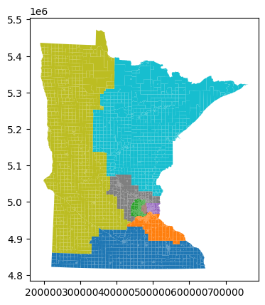
Of course, this isn’t very pretty, so let’s pass it some additional arguments to things a bit nicer:
fig, ax = plt.subplots(figsize=(8,8))
ax.set_yticks([])
ax.set_xticks([])
ax.set_title("Initial Partition in MN")
initial_partition.plot(ax=ax, cmap='tab20c')
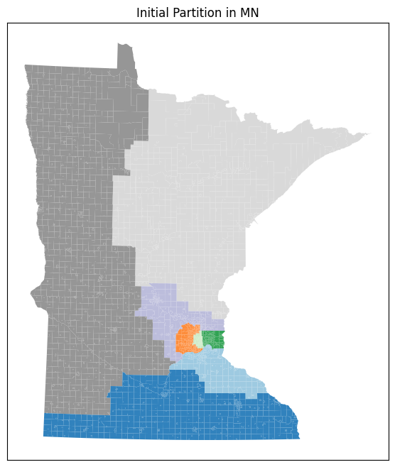
Under the hood, the plot method is using the geodataframe.plot method from
geopandas to plot the geometries, and all of this is
built on top of matplotlib, so most of the standard methods for modifying a
matplotlib plot will work here as well.
Now that we have our initial partition, we can run a Markov chain on it just as we have previously:
ideal_population = sum(initial_partition["population"].values()) / len(initial_partition)


proposal = partial(
    recom,
    pop_col="TOTPOP",
    pop_target=ideal_population,
    epsilon=0.01,
    node_repeats=2,
)

recom_chain = MarkovChain(
    proposal=proposal,
    constraints=[contiguous],
    accept=accept.always_accept,
    initial_state=initial_partition,
    total_steps=20,
)
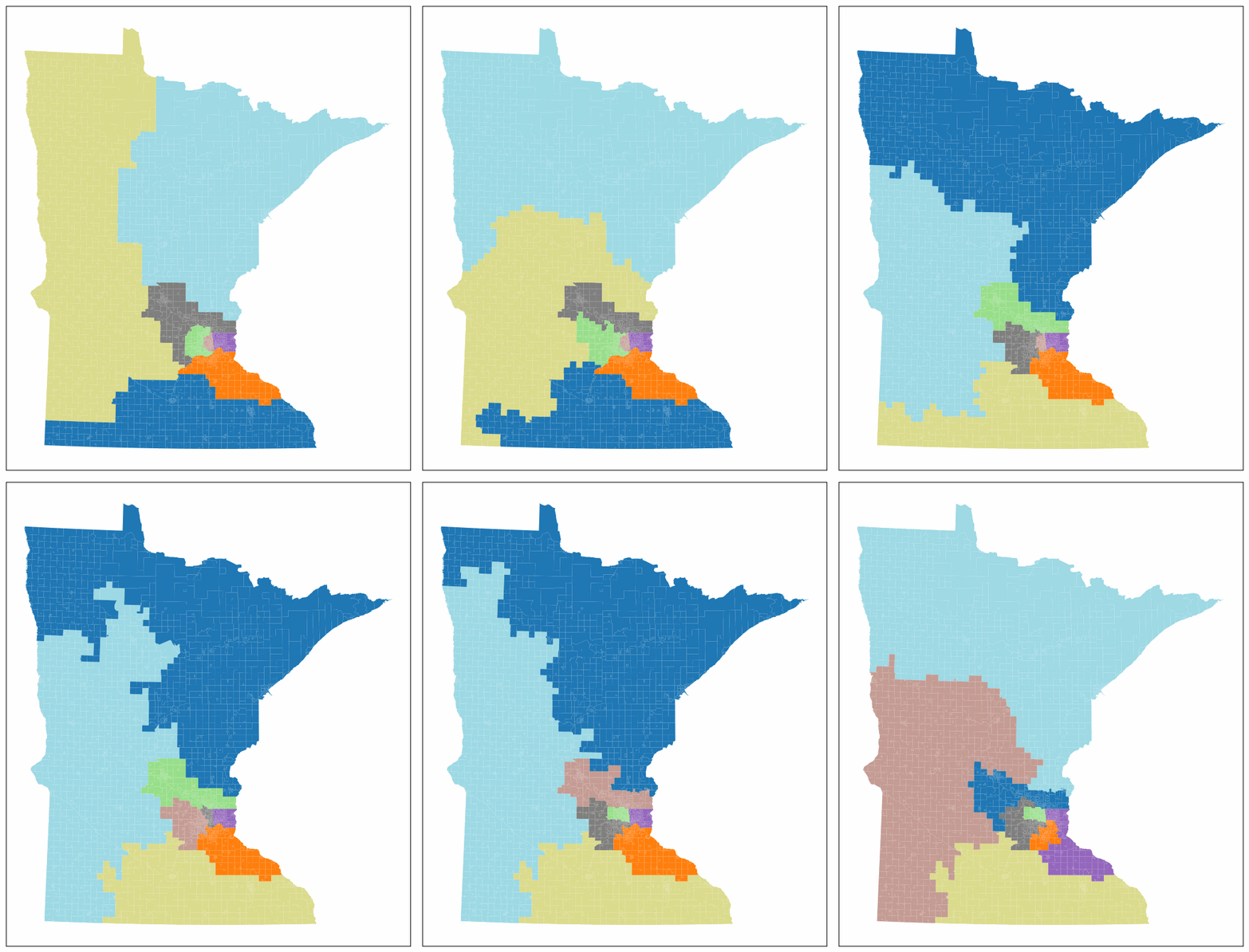
And the next bit of code will make a fun little widget that will allow us to watch the chain work!
%matplotlib inline
import matplotlib_inline.backend_inline
matplotlib_inline.backend_inline.set_matplotlib_formats('png')

import pandas as pd

import matplotlib.cm as mcm
import matplotlib.pyplot as plt
import networkx as nx
from PIL import Image
import io
import ipywidgets as widgets
from IPython.display import display, clear_output

frames = []
district_data = []

for i, partition in enumerate(recom_chain):
    for district_name in partition.perimeter.keys():
        population = partition.population[district_name]
        perimeter = partition.perimeter[district_name]
        area = partition.area[district_name]
        district_data.append((i, district_name, population, perimeter, area))

    buffer = io.BytesIO()
    fig, ax = plt.subplots(figsize=(10,10))
    partition.plot(ax=ax, cmap='tab20')
    ax.set_xticks([])
    ax.set_yticks([])
    plt.savefig(buffer, format='png', bbox_inches='tight')
    buffer.seek(0)
    image = Image.open(buffer)
    frames.append(image)
    plt.close(fig)

df = pd.DataFrame(
    district_data,
    columns=[
        'step',
        'district_name',
        'population',
        'perimeter',
        'area'
    ]
)

def show_frame(idx):
    clear_output(wait=True)
    display(frames[idx])

slider = widgets.IntSlider(value=0, min=0, max=len(frames)-1, step=1, description='Frame:')
slider.layout.width = '500px'
widgets.interactive(show_frame, idx=slider)
which should look something like this:
and our dataframe has collected all of the data we were interested in:
df.head(5)
step |
district_name |
population |
perimeter |
area |
|
|---|---|---|---|---|---|
0 |
0 |
8 |
662998.0 |
1.804646e+06 |
7.807545e+10 |
1 |
0 |
6 |
662979.0 |
6.616450e+05 |
7.864760e+09 |
2 |
0 |
5 |
662985.0 |
1.133867e+05 |
3.678103e+08 |
3 |
0 |
3 |
662994.0 |
2.625007e+05 |
1.509425e+09 |
4 |
0 |
7 |
662997.0 |
2.288428e+06 |
9.165192e+10 |